Introduction

It is often hard to train a model on predicting labels for a given set of data that will perform well on new sets of data as well. In machine laerning community, thus, Generalization is an important aspect of algorithms to handle unseen data and to make correct decision/prediction on them on running time. There are several ways to improve the generalization of a machine learning algorithm such as L1/L2 regularization (Ng, 2004), Dropout (Srivastava et al., 2014) for neural networks, etc.

On the other hand, training a new model on new datasets may also be infeasible due to challenges. Especially, it is difficult or even impossible to train a supervised model when there is a lack of labels for the new data. Acquiring a set of accurate labels for a new dataset is often challenging due to its nature of time and labor-intensive process.

One of possible approaches in such circumstances is domain adaptation, adapting a classifier trained using labeled samples in one domain (source domain) to classify samples in a new domain (target domain) while only a few of labeled samples in the new domain or none of them are available during training time. There have been early works in domain adaptation using subspace learning (Fernando et al., 2013), deep feature learning (Taigman et al., 2017), etc.

Liu et al. (2017) proposed the UNsupervised Image-to-image Translation (UNIT) framework that combines Variational Autoencoders (VAEs) (Kingma and Welling, 2014) and Genarative Adversarial Networks (GANs) (Goodfellow et al, 2014) with a shared-latent space assumption and they showed the UNIT framework can be utilized in domain adaptation problems. As an unsupervised method, however, the UNIT framework is expected to work only when the two domains have similar feature representations, e.g., visual look for images, for the same semantic classes. For example, the datasets used in their domain adaptation experiments, MNIST, USPS, and SVHN, are different datasets having different colors or lighting environment, but they are all Arabic numeral images which is the most critical visual characteristic in the class decision.

What if we need/want to apply domain adaption for datasets having totally different visual appearance for the same semantic classes? For example, MNIST and Kannada-MNIST, the datasets we will introduce shortly, are both handwritten digits datasets, but the former one contains Arabic numerals and the later one contains Kannada numerals.

In this project, we extend the UNIT framework to cope with the situations that the target domain classes have different visual representations and few/none of labeled samples. By introducing auxiliary classifiers into the framework, our proposed method is able to produce accurate image-to-image translation between the domains despite of their different visual appreance. Furthermore, our experimental results show that the proposed translator model gives higher classification accuracy than the baseline models trained on fully-labeled dataset for both domains.

MNIST and Kannada-MNIST

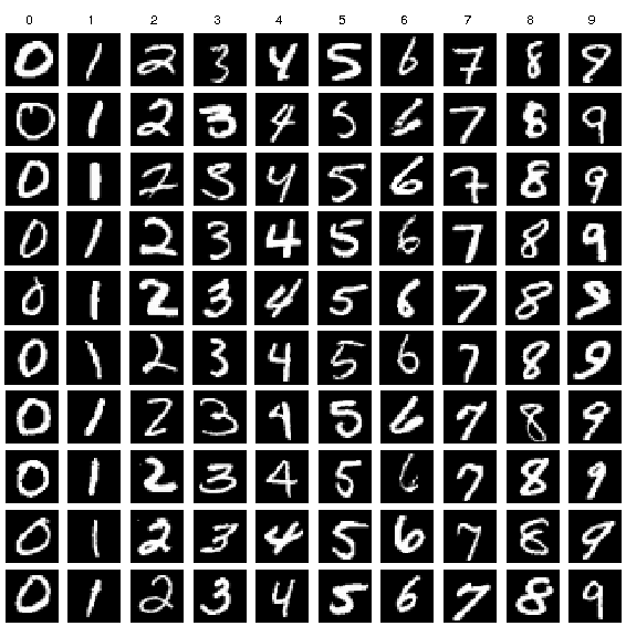
The MNIST dataset (LeCun et al., 2010) is one of the most commonly used dataset in machine learning research. This dataset consists of 70K images of size 28 pixels by 28 pixels. Each image contains a hand-drawn Arabic numeral between 0 to 9 inclusive. Due to its moderate size and label completeness, the MNIST dataset is widely used not only to train a handwritten digit recognition model but also as a benchmark dataset in developing many machine learning algorithms.

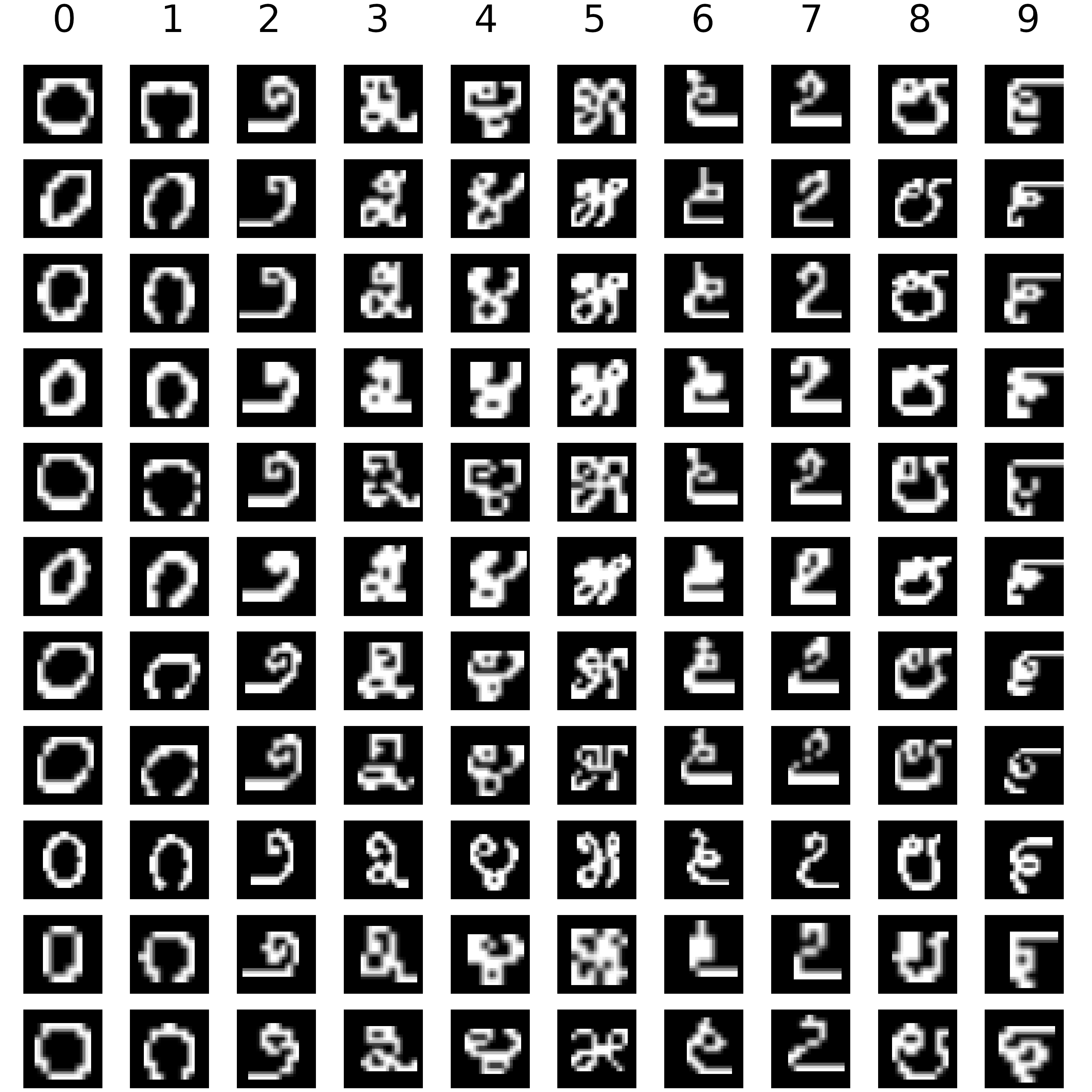
The Kannada-MNIST, or K-MNIST, dataset (Prabhu, 2019) is very similar to the MNIST dataset in terms of the number of samples and the size of each image except the images are of hand-drawn Kannada numerals instead of Arabic numerals. For reference, Kannada is a language predominantly spoken in Karnataka (a state in the southwest of India). This dataset is fairly new, and there are ongoing researches on how to train the most accurate model to predict the labels for this dataset.

Example images of MNIST and K-MNIST data for each numeric class are shown below. It is easy to notice that each digit representation is very different from each other, except 0, where Kannada numerals generally have more complicated strokes. Therefore, it is reasonable to assume that even a state-of-the-art MNIST classification model will have trouble on K-MNIST data.

MNIST	Kannada

Source: https://www.researchgate.net/figure/Example-images-from-the-MNIST-dataset_fig1_306056875	Source: https://towardsdatascience.com/a-new-handwritten-digits-dataset-in-ml-town-kannada-mnist-69df0f2d1456

Background

Variational Autoencoders

Autoencoders

In general, autoencoder is a form of unsupervised learning algorithm that implements the use of neural networks with the typical goal of data compression and dimensionality reduction.

Overall, the structure of an autoencoder can be outlined as follows:

Autoencoders
Autoencoder
Source: https://towardsdatascience.com/auto-encoder-what-is-it-and-what-is-it-used-for-part-1-3e5c6f017726

Encoder: a neural network responsible for reducing dimensionality of the input data
Bottleneck (latent space): the reduced vector representation of the input after the compression
Decoder: a neural network responsible for reproducing the original input from the bottleneck

Training of autoencoders typically done by minimizing the reconstruction loss, e.g., mean squared error, between the input and the output (the reconstructed input).

While autoencoders have been proven to be effective models for data compression, they cannot be used to generate new content just by having the decoder taking a sample vector from the latent space. This stems from the lack of regularization of the latent space by the autoencoder, whose learning and training processes direct towards the single goal of encoding and decoding the input. With the latent space constructed as distinct clusters by the encoder, thus exhibiting discontinuities, random sampling from such latent space and feeding it back into the decoder will result in non-meaningful output.

Variational Autoencoders

Variational Autoencoder (VAE) (Kingma and Welling, 2014) is a specific framework of “generative modeling” that deals with probabilistic distribution models of data points in the latent space. While structurally similar to an autoencoder, the encoder of VAE produces a distribution within the latent space rather than encoding a vector representation directly. This latent distribution is enforced to approximate a prior including but not limited to a normal distribution.

VAE
Variational Autoencoder
Source: https://towardsdatascience.com/understanding-variational-autoencoders-vaes-f70510919f73

The loss function of VAE can be represented as the negative log-likelihood with a regularization term. For each single data point $x_i$ , the loss function $\mathcal{L}_i$ is:

$\large \mathcal{L}_i(\theta, \phi; x_i) = - \mathbb{E}_{z \sim q_\theta (z|x_i)} [\log p_\phi (x_i | z)] + \mathbb{KL}[q_\theta(z|x_i) \Vert p(z)]$

where $\theta$ represents the encoder parameters and $\phi$ represents the decoder parameters.

The first term is basically the reconstruction loss which encourages the role of VAE as an ‘autoencoder’. On the other hand, the second term is the Kullback-Leibler (KL) divergence between the approximate posterior $q_{\theta} (z \vert x_i)$ and the latent prior $p(z)$ and it acts as a regularizer by forcing the latent distribution to be close to the prior. Please refer to (Kingma and Welling, 2014) for more details.

VAEs have been incorporated in literatures and practical scenarios for many different purposes, including but not limited to the interpolation of facial images with respect to different attributes such as age, hair color, expression, etc. (Yan et al., 2016)

Generative Adversarial Networks

Generative Adversarial Network (GAN) (Goodfellow et al, 2014) is another framework of deep-learning based generative models, which is widely used to translate inputs from one domain to another. While initially proposed as a model for unsupervised learning, GANs have been also proved to be useful for semi-supervised learning, fully supervised learning, and reinforcement learning.

Most GAN type of models involves two sub-models:

Generator (G): a neural network used to generate new examples from the problem domain.

The input to the model is a vector from a multidimensional space. After training with the dataset, this multidimensional space is mapped to corresponding points in the problem domain. This forms a compressed representation of the multidimensional data space.

After training, the generator model is used to generate new samples.
Discriminator (D): a neural network used to classify example inputs based on whether they come from the problem domain or from the generated examples.

The model inputs an example from the domain (real or generated) and classifies it with a binary label real or fake. The real examples come from the training dataset, while the fake examples come from the generator model.

Generative Adversarial Network
Source: (Hayes et al., 2019)

In terms of training a GAN, in essence, D and G play a two-player minimax game to optimize the expected value of the objective function:

$\large \begin{align} {\underset { G }{\operatorname { min } }} \; {\underset { D }{\operatorname { max } }} \quad & \mathbb{E}_{x \sim p_{\text{data}}(x)}[\log D(x)] + \mathbb{E}_{z_ \sim p(z)}[\log (1 - D(G(z)))] \end{align}$

where D is optimized to recognize the real and fake samples correctly while G is trained to fool the discriminator as much as possible by creating fake samples mimicking the real samples.

Image-to-Image Translation Networks

In this project, we use a framework that combines VAE and GAN to perform image-to-image translation tasks. Specifically, we adopt the UNIT framework proposed by Liu et al. (2017), which was used in unsupervised image-to-image translation tasks, while we further extend it to semi-supervised and fully-supervised image translation tasks.

Framework

The overall framework of our proposed model is depicted in the following figure.

SEMIT
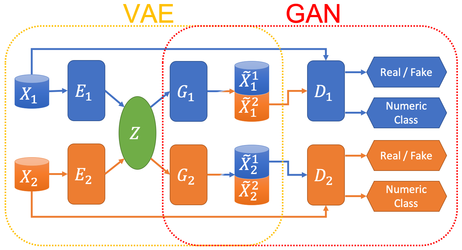
Image-to-image translation networks.

It is a combination of VAE and GAN architecture that consists of the following modules:

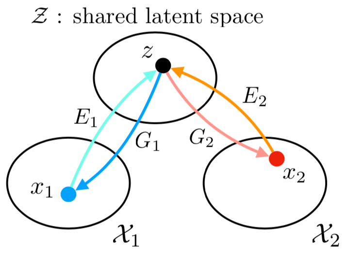
Encoders: each encoder $E_i$ encodes samples from a source domain data $X_1$ or a target domain data $X_2$ into a shared latent space^* $Z$ .
Decoders/Generators: each decoder (in terms of VAE) or generator (in terms of GAN) $G_i$ reconstructs samples $\widetilde{X}_{i}^{j}$ using latent vectors $z$ where the subscript $i$ means the decoder’s own domain and the superscript $j$ means the sample’s origin domain. For example, $\widetilde{X}_1^2$ represents the samples reconstructed in $X_1$ domain using the latent vectors encoded using the input data from $X_2$ domain.
Discriminators: each discriminator $D_i$ judges whether inputs are the real samples from the domain $X_i$ or fake (translated) samples, i.e., $\widetilde{X}_1^2$ or $\widetilde{X}_2^1$ . At the same time, each discriminator $D_i$ also gives class predictions for input samples, regardless of whether they are real or fake, similar to the one used in AC-GAN (Odena et al., 2017).

*Shared Latent Space

Source: Liu et al. (2017)

Since the latent space $Z$ is shared by both domains, it is possible to generate a target domain sample $\widetilde{x}_2$ from a latent vector $z$ that was encoded from a source domain sample $x_1$ , e.g., $\widetilde{x}_2=G_2(E_1(x_1))$ , or in the opposite direction.

All these modules are implemented as neural networks.

Training

In this section, we describe how the image-to-image translation model is trained.

Preliminaries

Assuming that we have two image data domain $X_1$ and $X_2$ , e.g., MNIST and K-MNIST, samples from each domain are drawn from each marginal distribution $P_{X_1}$ and $P_{X_2}$ .

In our translator model, the (variational) encoder outputs a mean vector $E_{\mu}(x)$ and a standard deviation vector $E_{\sigma}(x)$ . Thus, we represent the latent distribution $q$ and the latent codes $z$ drawn from this distribtuion as

$\large \begin{align} z_1 \sim q_1(z_1|x_1) &\equiv \mathcal{N}(z_1 | E_{1,\mu}(x_1), E_{1,\sigma}(x_1))\\ z_2 \sim q_2(z_2|x_2) &\equiv \mathcal{N}(z_2 | E_{2,\mu}(x_2), E_{2,\sigma}(x_2)) \end{align}$

according to the encoder input $x_1 \in X_1$ or $x_2 \in X_2$ . Furthermore, we use the reparameterization trick (Kingma and Welling, 2014) to enable backpropagation through the sampling operations of $z$ . On the other hand, we assume the standard normal distribution for the prior distribution of $z$ .

Loss and Objective Functions

There are three different types of loss functions used in training of our image-to-image translation models. Each loss function has its own objective according to the role of the corresponding modules in the entire model.

VAE Loss

First of all, the VAE losses are deployed to train the encoders $E_i$ and the decoders/generators $G_i$ to be able to reconstruct the samples from its own domain dataset $X_i$ using the stochastic samples $z$ from the shared latent space $Z$ . The VAE loss function for each domain can be written as follows:

$\large \begin{align} \mathcal{L}_{\text{VAE}_1}(E_1, G_1) &= \lambda_1 \text{KL}(q_1(z_1|x_1) \Vert p_\eta (z)) - \lambda_2 \mathbb{E}_{z_1 \sim q_1(z_1|x_1)}[\log p_{G_1} (x_1 | z_1)]\\ \mathcal{L}_{\text{VAE}_2}(E_2, G_2) &= \lambda_1 \text{KL}(q_2(z_2|x_2) \Vert p_\eta (z)) - \lambda_2 \mathbb{E}_{z_2 \sim q_2(z_2|x_2)}[\log p_{G_2} (x_2 | z_2)] \end{align}$

where the hyper-parameters $\lambda_1$ and $\lambda_2$ control the balance between the reconstruction error and the KL divergence of the latent distribution from its prior. We used fixed values of $\lambda_1 = 0.001$ and $\lambda_2 = 0.01$ in this project following the configuration used by (Liu et al., 2017).

GAN Objective

Next, GAN objectives are used to enforce the translated images look like images from the source domain through the adversarial training of generators and discriminators. For example, $D_1$ tries to discriminates the real samples $x_1 \sim X_1$ and the translated fake samples $\widetilde{x}_1^2 = G_1(z_2)$ . On the other hand, $G_1$ tries to make $D_1$ classify $\widetilde{x}_1^2$ as real samples. It can be formulated by following equations:

$\large \begin{align} \mathcal{L}_{\text{GAN}_1}(E_2, G_1, D_1) &= \mathbb{E}_{x_1 \sim P_{X_1}}[\log D_{1s}(x_1)] + \mathbb{E}_{z_2 \sim q_2(z_2|x_2)}[\log (1 - D_{1s}(G_1(z_2)))]\\ \mathcal{L}_{\text{GAN}_2}(E_1, G_2, D_2) &= \mathbb{E}_{x_2 \sim P_{X_2}}[\log D_{2s}(x_2)] + \mathbb{E}_{z_1 \sim q_1(z_1|x_1)}[\log (1 - D_{2s}(G_2(z_1)))] \end{align}$

where each $D_{is}$ refers to the discrimination output of $D_i$ .

Classification Loss

Finally, we also introduce the classification losses for the labeled samples, if any, to encourage matching the classes of the samples between two domains. For example, a translated sample $\widetilde{x}_1^2 = G_1(E_2(x_2))$ where $x_2$ has its label $y_2$ in the domain $X_2$ should be classified by $D_1$ as the same class in the domain $X_1$ . It can be formulated by cross-entropy loss or negative log-likelihood:

$\normalsize \begin{align} \mathcal{L}_{\text{CLASS}_1}(E_2, G_1, D_1) &= \alpha_1 \cdot {\underset { (x_1, y_1) \sim P_{X_{1}^{\text{labeled}}} }{\operatorname {\mathbb{E}} }}[−\log D_{1c}(y_1|x_1)] + \alpha_2 \cdot {\underset { z_2 \sim q_2(z_2|x_2), (x_2, y_2) \sim P_{X_{2}^{\text{labeled}}} }{\operatorname {\mathbb{E}} }}[−\log D_{1c}(y_2|G_1(x_2))]\\ \mathcal{L}_{\text{CLASS}_2}(E_1, G_2, D_2) &= \alpha_2 \cdot {\underset { (x_2, y_2) \sim P_{X_{2}^{\text{labeled}}} }{\operatorname {\mathbb{E}} }}[−\log D_{2c}(y_2|x_2)] + \alpha_1 \cdot {\underset { z_1 \sim q_1(z_1|x_1), (x_1, y_1) \sim P_{X_{1}^{\text{labeled}}} }{\operatorname {\mathbb{E}} }}[−\log D_{2c}(y_1|G_2(x_1))] \end{align}$

where $\alpha_i$

$\large \alpha_i = \eta \cdot \frac{\text{the number of all samples in } X_i}{\text{the number of labeled samples in } X_i}$

and $\eta$ is a hyper-parameters that controls the weight of classification loss. We use $\eta=1$ as a default value in this project.

Joint Optimization

Combining the losses and objective functions above together, we jointly optimize the following minimax problem:

$\large \begin{align} {\underset { E_1, E_2, G_1, G_2 }{\operatorname { min } }} \;\; {\underset { D_1, D_2 }{\operatorname { max } }} \quad & \mathcal{L}_{\text{VAE}_1}(E_1, G_1) + \mathcal{L}_{\text{GAN}_1}(E_2, G_1, D_1) + \mathcal{L}_{\text{CLASS}_1}(E_2, G_1, D_1)\\ + &\mathcal{L}_{\text{VAE}_2}(E_2, G_2) + \mathcal{L}_{\text{GAN}_2}(E_1, G_2, D_2) + \mathcal{L}_{\text{CLASS}_2}(E_1, G_2, D_2) \end{align}$

We use an alternating training procedure to solve this. Specifically, we first update $D_1$ and $D_2$ by applying a (stochastic) gradient ascent step while the parameters of the other modules are fixed. Then, $E_1, E_2, G_1,$ and $G_2$ are updated with a gradient descent step while $D_1$ and $D_2$ are fixed.

Experiments

We conducted various experiments to answer the following questions:

Is our translator model able to translate images to the source domain?
Are the translated images can be classified correctly by the source domain classifier model?
Is the shared latent space actually meaningful?

All experiments are done with Python 3.7 with several packages including PyTorch and TensorFlow. All source codes are available at our project GitHub repository.

Setup

Dataset Preparation

Source and Target Domain

We used MNIST as our source domain and K-MNIST as our target domain. In other words, our model aims to translate images of Kannada numerals to ones that look like typical Arabic numerals for domain adaptation.

Amount of Supervision

Assuming that a well-studied source domain dataset is available, we use the complete MNIST dataset with all labels. On the other hand, we do experiments with several possible scenarios regarding the target domain dataset. Specifically, we compare the classification accuracy of the translated images when we use the K-MNIST training set with no labels, partial labels, and all labels.

Preprocessing

We use resized 32x32 images for the development convenience which are then normalized to the range of [0, 1] by default. Our translator models use shifted and re-scaled data whose range is [-1, 1].

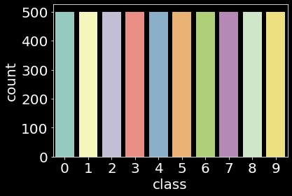
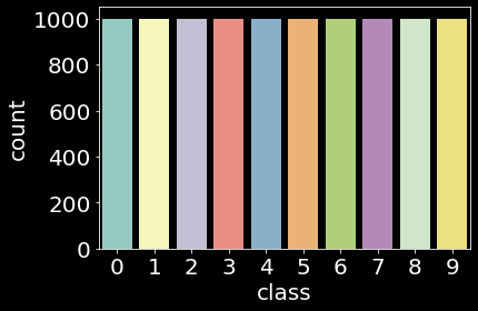
Train / Validation / Test Splits

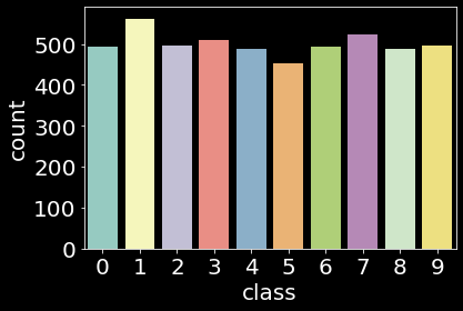
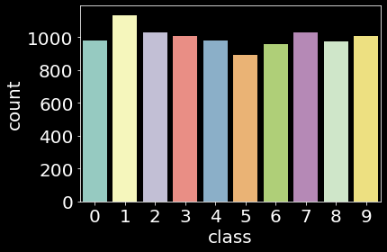
While we use the original splits of 60K training set and 10K test set for both dataset, we extract 5K samples as a validation set from each training set by using stratified random sampling.

Dataset	Train	Validation	Test
MNIST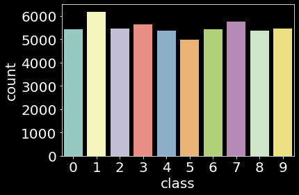
Kannada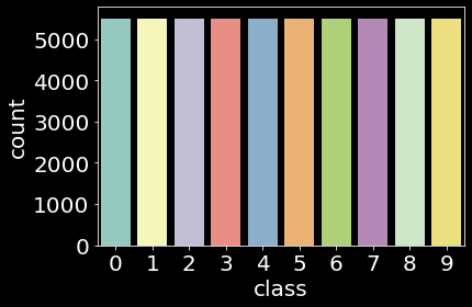

Model Architecture

All modules in our image-to-image translator are based on convolutional neural networks. The architecture of each module is summarized in the table below, where Nx is the number of filters in a convolutional (Conv2D) or transposed convolutional (TransConv2D) layer or the number of hidden units in a fully-connected (FC) layer, Kx is the kernel size, Sx is the stride size, and Px is the padding size. We use Batch Normalization (Ioffe et al., 2015) after each layer in the encoder and generator, and Dropout (Srivastava et al., 2014) of 0.5 drop rate after each layer in the discriminator. Leaky ReLU (Maas et al., 2013) activation function is mainly used except the last layers of the modules.

Layer	Encoder	Decoder/Generator	Discriminator
1	Conv2D(N32, K4, S2, P1) - BatchNorm - LeakyReLU	TransConv2D(N512, K4, S2, P1) - BatchNorm - LeakyReLU	Conv2D(N32, K4, S2, P1) - LeakyReLU - Dropout
2	Conv2D(N64, K4, S2, P1) - BatchNorm - LeakyReLU	TransConv2D(N256, K4, S2, P1) - BatchNorm - LeakyReLU	Conv2D(N64, K4, S2, P1) - LeakyReLU - Dropout
3	Conv2D(N128, K4, S2, P1) - BatchNorm - LeakyReLU	TransConv2D(N128, K4, S2, P1) - BatchNorm - LeakyReLU	Conv2D(N128, K4, S2, P1) - LeakyReLU - Dropout
4	Conv2D(N256, K4, S2, P1) - BatchNorm - LeakyReLU	TransConv2D(N64, K4, S2, P1) - BatchNorm - LeakyReLU	Conv2D(N256, K4, S2, P1) - LeakyReLU - Dropout
5	Conv2D(N512, K4, S2, P1) - BatchNorm - LeakyReLU	TransConv2D(N32, K4, S2, P1) - BatchNorm - Tanh	Conv2D(N512, K4, S2, P1) - LeakyReLU - Dropout
6a	$\mu$ : Conv2D(N512, K1, S1, P0)		Real/Fake: FC(N1) - Sigmoid
6b	$\sigma$ : Conv2D(N512, K1, S1, P0) - Softplus		Class: FC(N10) - Softmax

The model parameters were optimized with Adam (Kingma and Ba, 2015) optimizer with the learning late of 0.0002 and the momentum of $\beta_1 = 0.5$ and $\beta_2=0.999$ . Our translator models were trained over 100 epochs with mini-batchs of 64 samples.

Baseline Classifiers

We compared the classification accuracy of our translator model to a baseline classification model for each dataset. Each baseline classifier resembles the discriminator module in our translator model except there is no source discrimination (real/fake) head in the last layer. Each baseline classifier is trained using either dataset only, and thus it is expected to perform well only for the domain where it was trained. On the other hand, our translator model is trained using both datasets regardless of the number of labeled training samples from the target domain; therefore, we expect that our translator well classifies samples from both domains using the discriminators $D_1$ or $D_2$ .

These comparisons allow us to ultimately determine whether our translator model could translate Kannada numeral images to Arabic ones (and vice versa) effectively.

Results

Validation of VAE Module

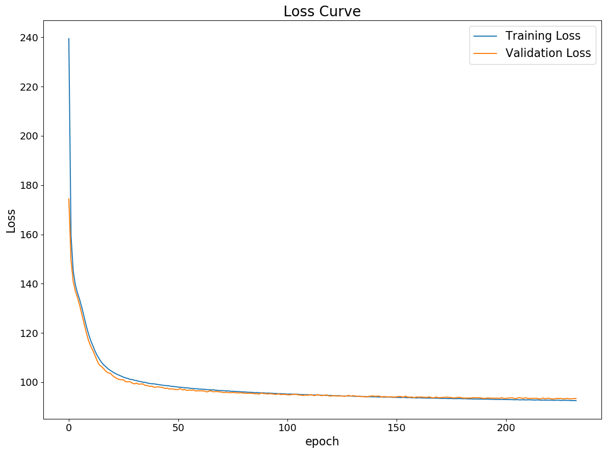
As the foremost step of the entire project, we trained and evaluated the VAE module, a set of the encoder and the generator, for each dataset independently first since it is a core of our translator model. The VAE loss values over about 200 epochs of training for each dataset are shown below.

MNIST	K-MNIST

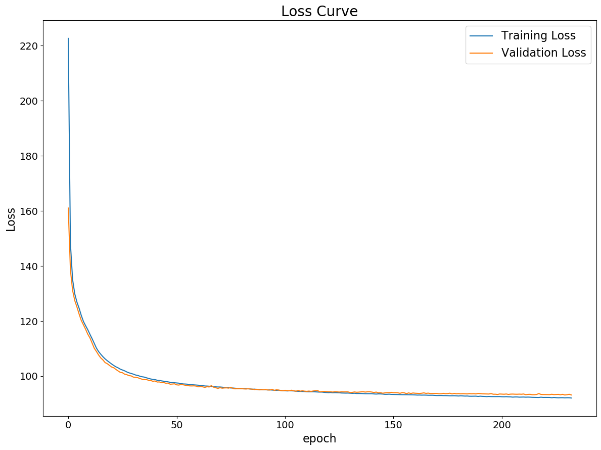We confirmed that the VAE module is trained and perform well on both datasets with neither overfitting nor underfitting.

Translation

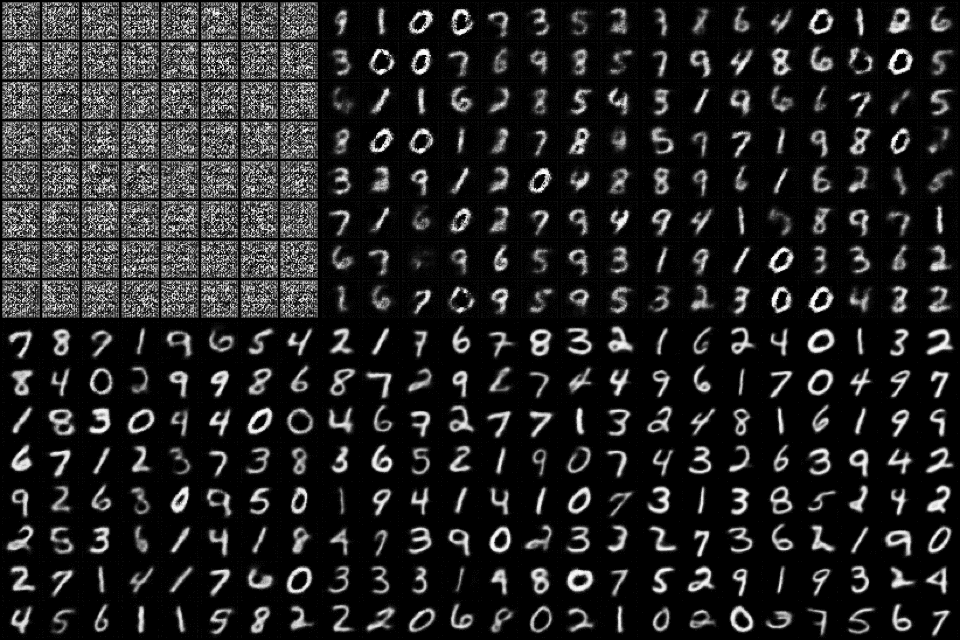
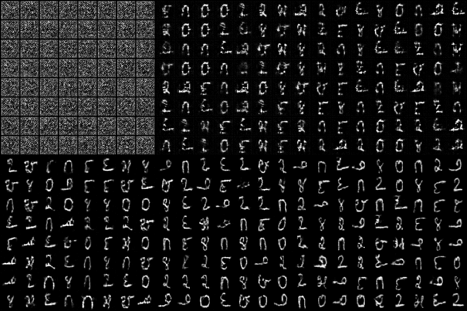
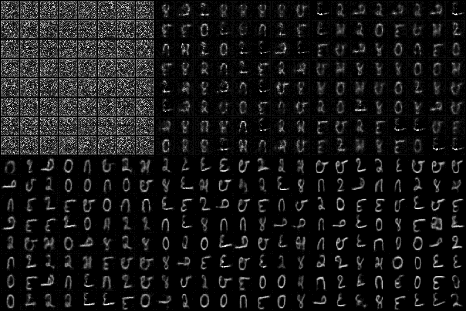
To answer the first main question at the beginning of this section, we show how our model successfully translate the images. Visual representations of our translation between Kannada numerals (K-MNIST) and Arabic numerals (MNIST) are shown in the table below. For each dataset (row), each column contains a GIF image as a progress recording over the training epochs for the followings:

The first column shows the input images to our model:
$\large x_1 \sim X_1$ (MNIST) or $x_2 \sim X_2$ (K-MNIST)
The second column shows the reconstructed images by the VAE modules for each domain itself:
$\large \widetilde{x}_1^1 = G_1(E_1(x_1))$ or $\widetilde{x}_2^2 = G_2(E_2(x_2))$
The last column contains the translated images between the domains:
$\large \widetilde{x}_1^2 = G_2(E_1(x_1))$ or $\widetilde{x}_2^1 = G_1(E_2(x_2))$

Dataset	Input $X_i$	Reconstruction $X_i \rightarrow \widetilde{X}_i^i$	Translation $X_i \rightarrow \widetilde{X}_j^i$
MNIST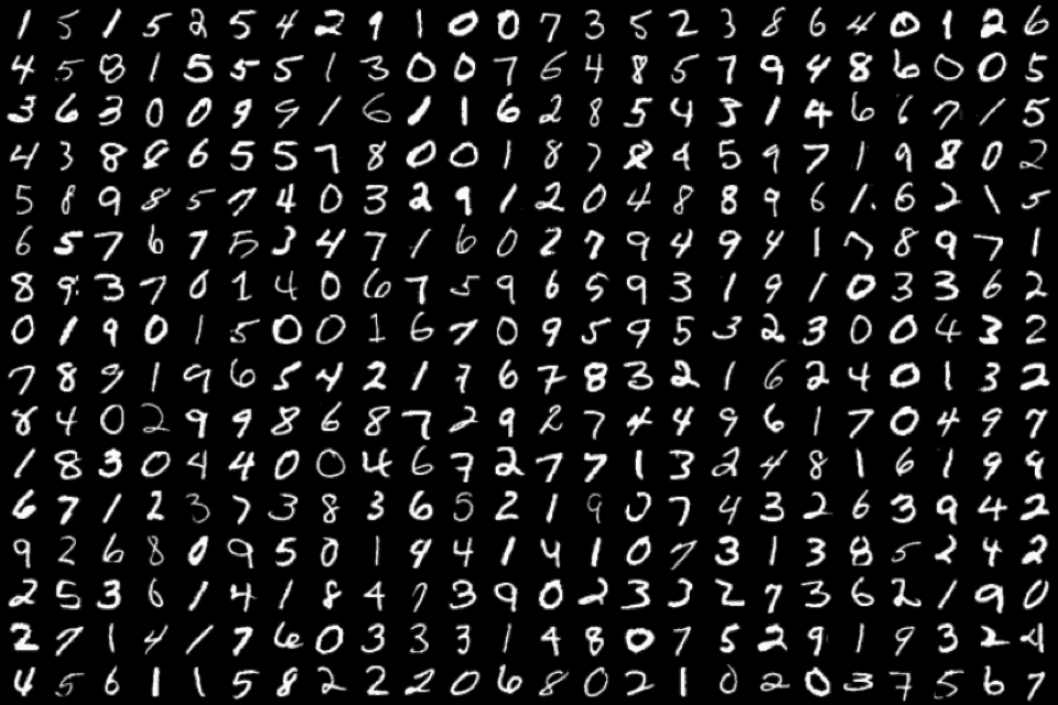
K-MNIST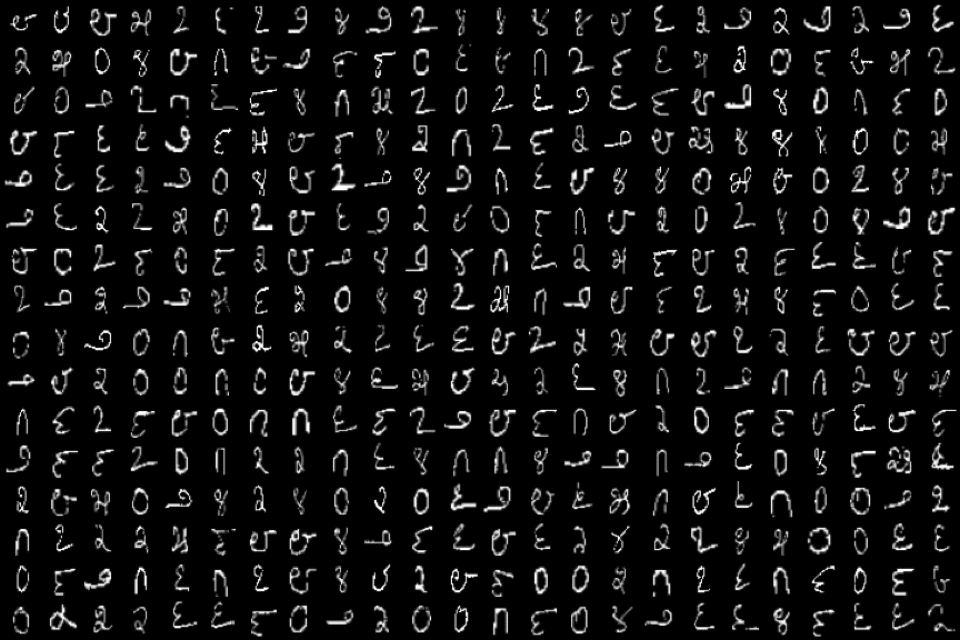

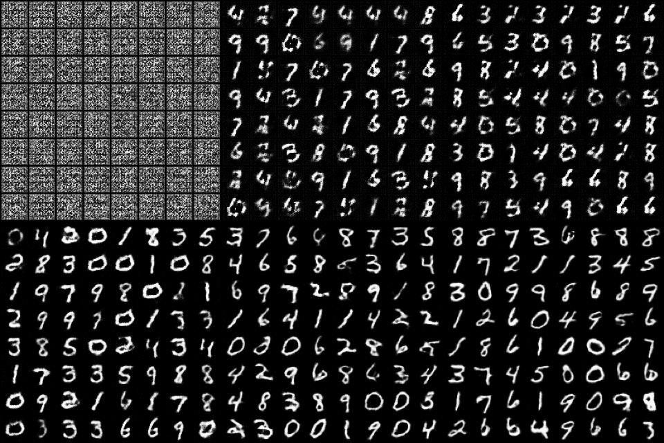It is shown that our model gives poor outputs that look like noise for both reconstruction and translation in the early stage of the training. However, they become very clear and realistic as the training progress. We can see that our translator model performs well on both direction of translation, MNIST $\rightarrow$ K-MNIST and K-MNIST $\rightarrow$ MNIST.

Classification Performance

Next, we investigated whether the translated images can be classified correctly by the translator itself. Please note that our translator model already contains a classifier for each domain as a classification head of the discriminator. Therefore, we do not need to train a classifier for the translated images from scratch.

We used the discriminator of MNIST domain, $D_1$ , to classify the images in both datasets. While the MNIST images were fed into $D_1$ directly, $\hat{y}_1 = D_1(x_1)$ , for the validation purpose, K-MNIST images were translated to MNIST domain first before classifying them, $\hat{y}_2 = D_1(G_1(E_2(x_2)))$ . On the other hand, Dig-MNIST test set, which is a difficult version of K-MNIST test set, was also evaluated as an extended comparison.

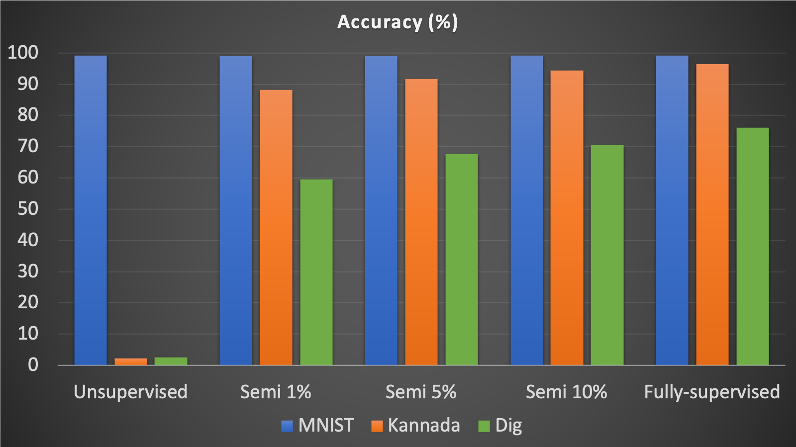
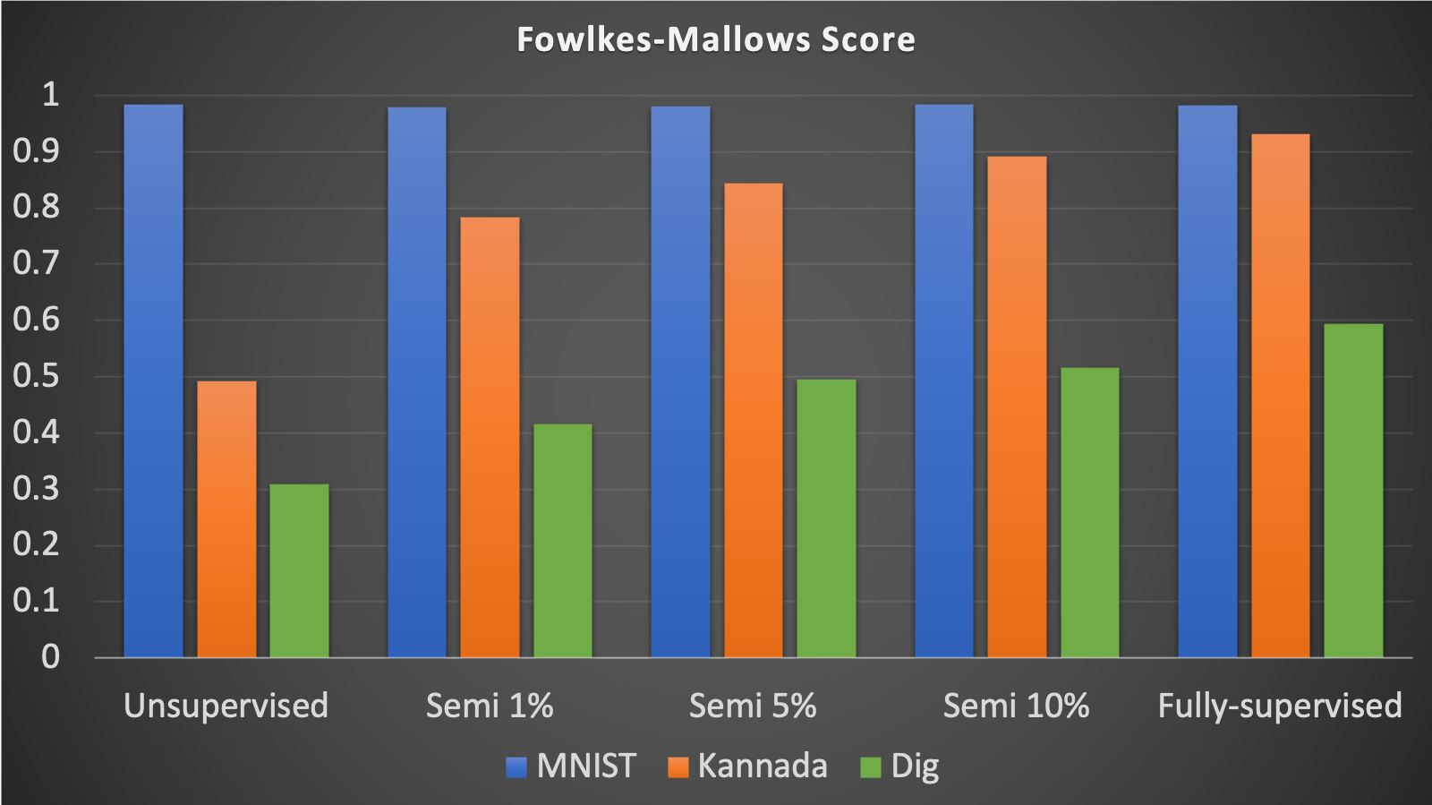
We compared the classification performance of 5 different translators trained by different amounts of the labels (supervision) for K-MNIST while all labels were used for MNIST. While the accuracy were used as the main metric of comparisons, we also calculated Fowlkes-Mallows Score to see how unsupervised translator performs. The comparison results are summarized in the charts below.

All different translators classify MNIST images well with a high accuracy of about 99%, which was expected because we used all labels for MNIST images.

On the other hand, the accuracy of our K-MNIST data translation increases from unsupervised learning to fully supervised learning. Using unsupervised learning for K-MNIST translation, our accuracy was about 3%, showing that our model couldn’t translate images effectively. However, as Fowlkes-Mallows score shows, there are still some well-formed clusters. We can infer from this that there exists some mapping between K-MNIST class and MNIST class even though their numeric values are not matched due to the lack of supervision by labels.

With a 1% semi-supervised learning, the accuracy increased tremendously for K-MNIST data translation – the accuracy was about 88%. This shows that even with a small amount of labeled data, our model can translate at a greater performance. This is further shown with the increase in accuracy for 5% semi-supervised learning (accuracy is about 92%) and for 10% semi-supervised learning (accuracy is about 94%). The highest accuracy achieved with K-MNIST data translation was about 96% accuracy. This was achieved with fully-supervised learning. Therefore, with more labeled data, our model can translate Kannada MNIST data better.

The same trend also occurred for Dig-MNIST data. The accuracy showed an increasing trend as the learning became more supervised from 3% for the unsupervised translation to 76% for the fully-supervised translation.

Meanwhile, we also compared the accuracy of our translator model to the aforementioned baseline classification models as well as some state-of-the-art results, which are summarized in the following table:

Model	MNIST	K-MNIST	Dig-MNIST
1% semi-supervised	98.95	88.16	59.49
5% semi-supervised	99.03	91.64	67.71
10% semi-supervised	99.19	94.37	70.49
Fully-supervised	99.09	96.45	76.12
Our MNIST Baseline	96.73	20.74	16.99
Our K-MNIST Baseline	24.21	95.33	72.59
MNIST State-of-the-art (Byerly et al., 2020)	99.84	-	-
K-MNIST Kaggle 1st place	-	99.6	-

Since the baseline classifiers were trained on each dataset only, they perform very poor on the other domain. On the other hand, our translator model performs well on both domain. Furthermore, our translator performs even better than the baseline classifier for each domain. It can be inferred that the translation task helps on regularization and thus the translator model generalizes well on the classification taks as well.

There is still room for improvements as the accuracy of translator is behind the state-of-the-art classification model for each dataset. We expect the performance of both translation and classification can be further improved if we adopt more sophisticated architectures for our backbone modules of the encoder, generator, and discriminator.

Visualization of the Shared Latent Space

Last but not least, we visualized the shared latent space learned by our translator model. We collected all latent vector $z$ from both datasets using the encoders $E_1$ and $E_2$ and construct 2-dimensional visualization embeddings using t-SNE (Maaten 2014).

The visualization below shows that the most corresponding digits of Kannada and Arabic numbers, except 0 and 6, are adjacent to each other in the shared latent space learned. This represents the clustered relationships between two different domains that enable translations between them.

There does exist a lack of close connections across the domains for the two numerals, 0 and 6, in the shared latent space. This might be a possible reason as to why the classification accuracy of K-MNIST after translation is not same as MNIST; the translator might have difficulties on translating them due to the lack of the connections.

tSNE
t-SNE visualization of the shared latent space

Conclusion

In this project, we designed a novel (semi-)supervised image-to-image translator using neural networks. It was shown that our translator model was able to translate images between two domains, from K-MNIST to MNIST and vice versa, effectively. Our translator model can also directly classify the images from both domains. Furthermore, our translator model can be trained with even a small amount of labels for the dataset to be translated. It was enabled by the shared latent space that connects two different data domains together, which was visually confirmed.

References

(Ng, 2004) Ng, Andrew Y. “Feature selection, L 1 vs. L 2 regularization, and rotational invariance.” Proceedings of the twenty-first international conference on Machine learning. 2004.
(Fernando et al., 2013) Fernando, Basura, et al. “Unsupervised visual domain adaptation using subspace alignment.” Proceedings of the IEEE international conference on computer vision. 2013.
(Taigman et al., 2017) Taigman, Yaniv, Adam Polyak, and Lior Wolf. “Unsupervised cross-domain image generation.” International Conference on Learning Representations (ICLR), 2017.
(Liu et al., 2017) Liu, Ming-Yu, Thomas Breuel, and Jan Kautz. “Unsupervised image-to-image translation networks.” Advances in neural information processing systems. 2017.
(Kingma and Welling, 2014) Kingma, Diederik P., and Max Welling. “Auto-encoding variational bayes.” International Conference on Learning Representations (ICLR), 2014.
(Goodfellow et al., 2014) Goodfellow, Ian, et al. “Generative adversarial nets.” Advances in neural information processing systems. 2014.
(LeCun et al., 2010) LeCun, Y., Cortes, C., and Burges, C. Mnist handwritten digit database. ATT Labs [Online], 2010.
(Prabhu, 2019) Prabhu, Vinay Uday. “Kannada-mnist: A new handwritten digits dataset for the kannada language.” arXiv preprint arXiv:1908.01242 (2019).
(Yan et al., 2016) Yan, Xinchen, et al. “Attribute2image: Conditional image generation from visual attributes.” European Conference on Computer Vision. Springer, Cham, 2016.
(Hayes et al., 2019) Hayes, Jamie, et al. “LOGAN: Membership inference attacks against generative models.” Proceedings on Privacy Enhancing Technologies 2019.1 (2019): 133-152.
(Odena et al., 2017) Odena, Augustus, Christopher Olah, and Jonathon Shlens. “Conditional image synthesis with auxiliary classifier gans.” Proceedings of the 34th International Conference on Machine Learning-Volume 70. JMLR. org, 2017.
(Byerly et al., 2020) Byerly, Adam, Tatiana Kalganova, and Ian Dear. “A Branching and Merging Convolutional Network with Homogeneous Filter Capsules.” arXiv preprint arXiv:2001.09136 (2020).
(Ioffe et al., 2015) Ioffe, Sergey, and Christian Szegedy. “Batch normalization: Accelerating deep network training by reducing internal covariate shift.” arXiv preprint arXiv:1502.03167 (2015).
(Srivastava et al., 2014) Srivastava, Nitish, et al. “Dropout: a simple way to prevent neural networks from overfitting.” The journal of machine learning research 15.1 (2014): 1929-1958.
(Maas et al., 2013) Maas, Andrew L., Awni Y. Hannun, and Andrew Y. Ng. “Rectifier nonlinearities improve neural network acoustic models.” ICML Workshop on Deep Learning for Audio, Speech, and Language Processing (WDLASL), 2013.
(Dugas et al., 2001) Dugas, Charles, et al. “Incorporating second-order functional knowledge for better option pricing.” Advances in neural information processing systems. 2001.
(Kingma and Ba, 2015) Kingma, Diederik P. and Jimmy Ba. “Adam: A Method for Stochastic Optimization.” International Conference on Learning Representations (ICLR), 2015.
(Maaten 2014) Van Der Maaten, Laurens. “Accelerating t-SNE using tree-based algorithms.” The Journal of Machine Learning Research 15.1 (2014): 3221-3245.